Creating a Budget, Part 3

This is a series for creating a budget using Google Docs. Part One and Part Two describe creating a basic budget form.

In Part Two, we completed our Google Document Budget Spreadsheet. Now, you should test out the formulas that we entered and make sure that everything is working.

Go ahead, take some time to fill in the numbers. Don’t worry, if this is your first budget, it will not be accurate for about the first three months. After that, budgeting becomes second nature.

Allocating Your Income

Congratulations! You have just completed your first Zero Based Budget! You have spent EVERY penny on paper, on purpose before the month has begun. You want to do this every month. Cindy and I recommend that you start about mid-month so that you can forecast all of the monthly variables (such as Valentine’s Days, birthdays and kids needing clothing).

Next, we want to allocate your income over the next month. Life would be simple if we could get one paycheck at the start of the month and we could execute on the budget, but most of us get paid on a varying cycle.

In my household, we have only one regular income, which occurs bi-weekly. The biggest category on my budget is the mortgage. If I pay for my mortgage out of one paycheck, it will leave very little left over for other necessities, so, I am going to take half out of each paycheck.

With your Spreadsheet open, we are going to add to our column headers:

I have added a Pay Date, an Income and an Allocated Column. The Income Column and the Allocated Column are going to save the same purposes as cells B2 and C2.

Next, just like in the budget side, we are going to merge cells. However, instead of two columns, we are going to merge three:

Finally, we are going to add a formula to the allocated cell at F2: E2 -SUM(D3:D26).

Note: When you merge cells, you address the values in formulas using the left most cell. That is why we use SUM(D3:D26) instead of SUM(F3:F26).

Complete the new columns by adding formatting to the headers. If you have any other income that occurs on other dates, add another set of columns.

I copied and pasted the columns from D – F, but I had to re-enter the formula because the cell references where not correct. Make sure you enter some values to test that the Allocated values are working correctly.

Making Sure it all Adds Up

The last thing that I want to add to this are columns that will help me to determine that I have allocated everything correctly.

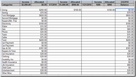
The formula for the first row is as follows: =B3-SUM(D3:G3). To translate what this is doing: subtract the value of cell B3 from the Sum of Cells D3 and G3 (technically, this says to sum all cells between D3 and G3). I am going to place this formula into cell J3 and then will copy this all the way down to my last category:

I’ve also created a header.

Now the completed spreadsheet looks like this:

Just a note – I do not use Google Docs for my spreadsheet – I use Excel. I have found that entering formulas into Google and copying cells is not as forgiving as Excel, but, as a free alternative, Google Docs is pretty good.

I hope that this series helps you get a very simple way of creating a zero based budget and allocation plan.